Kinetica Sparse Data Tutorial

Introduction

This tutorial describes the application of Singular Value Decomposition or SVD to the analysis of sparse data for the purposes of producing recommendations, clustering, and visualization on the Kinetica platform. Sparse data is common in industry and especially in retail. It often results when a large set of customers make a small number of choices from a large set of options. Some examples include product purchases, movie rentals, social media likes, and election votes.

The SVD approach to analyzing sparse data has a notable history of success. In 2006 Netflix hosted a million dollar competition for the best movie recommendation algorithm and most of the leading entries used SVD. It also inspired the techniques used by Cambridge Analytica when they assisted Trump in the 2016 presidential election.

We will leverage Python and Jupyter notebooks with some ML libraries including Scikit Learn and PyTorch. Data will be persisted in Kinetica tables and we will use Kinetica for calculating dot products necessary for inferencing.

We start by downloading a sample dataset of Amazon product ratings that will be used to construct a sparse matrix. We will use SVD to decompose the matrix into singular vectors to build a recommender. Finally we will use the singular vectors for clustering and visualization.

This tutorial attempts to exclude some details of the linear algebra concepts. If you don’t know linear algebra then you can still benefit from this tutorial but if you do then you should first review the more technical explanations in ML Techniques for Sparse Data.

Prerequisites

This tutorial is based on prior work described in the Kinetica with JupyterLab Tutorial so if you have not already completed this tutorial then you should do this first.

The Docker image is loaded with all the dependencies needed which include:

• Kinetica 6.2
• JupyterLab
• Python 3.6
• PyTorch
• Pandas
• Scikit Learn

Concepts

The Sparse Data Problem

We will begin with a common sparse data analysis problem which involves customer purchasing data for a retail business. When we analyze this type of data we want to find patterns in customer behavior so we can group them into categories, make predictions, and detect anomalies.

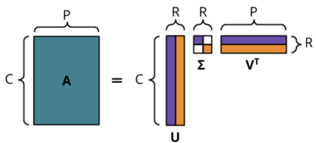
We can take a historical record of customer purchases and generate a table where the rows are customers and the columns are actions or purchases. For example the table below shows the purchases for a hypothetical store with C customers and P products. The data in this table has dimensions of C x P.

[table id=3 /]

Each cell indicates the quantity of a product the customer purchased. If no product was purchased then the cell is empty. Because the table is generated from purchase activity there should be no empty rows or columns.

The table can be represented with the following sparse matrix where empty values are assigned to zero.

In a real world scenario a matrix like this will have tens of thousands of rows and columns. Most of the values will be empty because customers typically purchase only a few of the available products. When we have a data structure where most of the values are empty we say that it is sparse.

Sparse data presents a problem for many analysis techniques and one approach is to leverage methods that can produce a compressed representation of the matrix and express it in a different form using less data.

During the compression process important patterns are identified and used to build a simplified representation while noise or data that does not fit identified patterns is eliminated.This is often called dimensional reduction because we express the matrix with less dimensions (or lower rank) while preserving its most significant features.

The SVD Solution

Singular Value Decomposition or SVD, is a traditional and effective approach involving iterative solvers that first emerged in the 1960s. It uses matrix factorization to break up a matrix into 3 smaller matrices that allow for control over the extent of the dimensional reduction. It does this by breaking up the data into principal component vectors. We can use the resulting matrices to dimensionally reduce the dataset by keeping only the most significant vectors.

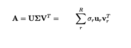
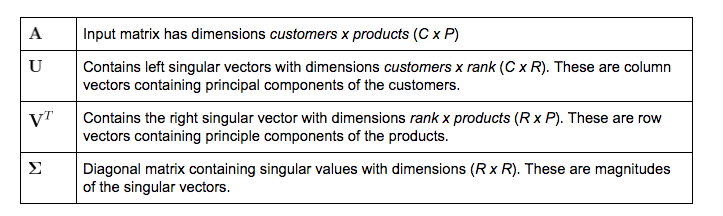
Below is the SVD equation showing the three component matrices that are provided by the solver.

• The   matrix contains row vectors for each customer
• The  matrix contains column vectors for each product
• The   matrix contains magnitudes of the vectors in descending order.
• Using these components we can reconstruct the original matrix A with with as little or as much detail as we want.

Sparse Data Visualization

Clustering algorithms struggle with sparse data because of its high dimensionality but the reduced rank results from SVD allow us to cluster on more dense and compressed data. For example we might want to group customers by buying patterns or group products that are often purchased together.

We can use the k-means clustering algorithm to partition the the SVD customer vectors into a specified number of clusters. Each cluster has a centroid that represents the mean of the customer vectors and can be handled like a representative customer for the cluster. We can use these centroids to get descriptions for each cluster.

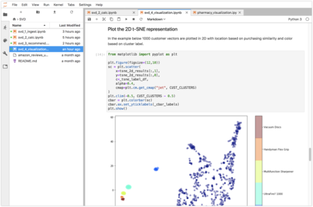
We can then visualize sparse data from the clustering results on a 2D or 3D map that represents similarity by position and clustering by class break. In the example below 1000 pharmacy patients are plotted based on their drug purchases. The color indicates the drug purchasing cluster and the location indicates the purchasing similarity.

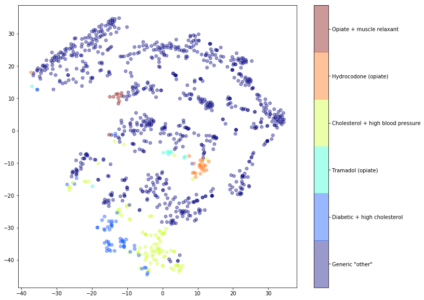
We can see that the k-means has identified a group for patients who purchase drugs for Cholesterol + high blood pressure and a another for Diabetic + high cholesterol. These clusters are located next to each other (see the blue and yellow points) indicating similarities between the two groups.

Running the Notebooks

Accessing the Notebooks and Data

At this point you should have the JupyterLab docker image running. Open the UI with http://localhost:8888/, use password kinetica, and navigate to the SVD folder.

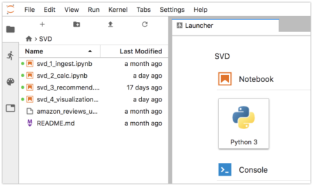
There are four notebooks that we will use in the tutorial:

[table id=5 /]

These notebooks have outputs that were saved from a previous run. Clear the outputs with Edit->Clear All Outputs. To run cells one at a time select the first cell and click the Play ▶ button. Variables are saved in the notebook’s kernel so you can edit and re-run any cell.

Each of the notebooks should run without modification or configuration. These notebooks also contain their own documentation so the contents of this tutorial can be considered supplemental.

You can access GAdmin http://localhost:8080/ with login admin/admin.

1. Ingest Data From Amazon

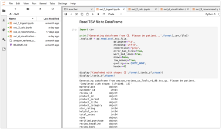
We will be ingesting data from the Amazon Customer Reviews Dataset that consists of over 130 million customer reviews from 1995 until 2015. The data we will be downloading is a TSV separated file. There are numerous different categories of product reviews and we will be ingesting data from the Tools category. A full index of categories is available if you want to change this.

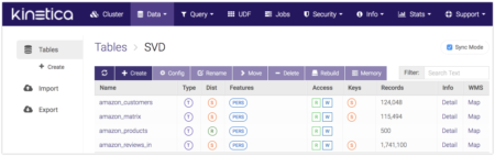
The file to download is 338MB containing 1.7 million reviews so it may take a while to run. It will be saved to the SVD directory with the notebooks. After that we read it to a dataframe, do some data cleansing, and save it to a table named amazon_reviews_in. The tables generated will be the following:

[table id=6 /]

The most important table is amazon_matrix that we will be using to generate the sparse matrix in our analysis. You can review the data from within GAdmin.

2. Execute SVD Analysis

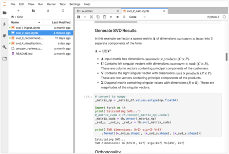
The next step is to construct a sparse matrix from amazon_reviews_in and generate the SVD matrix decomposition. To to this we load the table into a dataframe and pivot it into a sparse matrix that has dimensions of 65531 customers by 497 products.

The sparse matrix will be passed to the PyTorch solver. We truncate the U and V matrices to rank 10, multiply the  values into the matrices and save the resulting 10-dimensional vectors to tables. Finally, we do a comparison of the actual and approximate data.

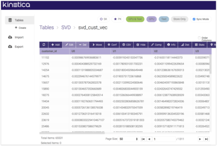
[table id=7 /]

The resulting tables contain 10 numbers for each customer and product. These numbers don’t mean much by themselves but when the vectors multiplied together they give an simplified approximation of the original data.

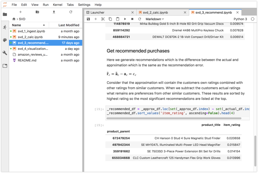
3. Test a Recommendation Scenario

In this step we use the SVD data from the previous step to compute a set of product recommendations for a single customer. This computation requires a set of dot products and we don’t need any ML libraries for it because the dot products are calculated directly by Kinetica in SQL. When running in a GPU enabled instance Kinetica will leverage the GPU for parts of the SQL execution.

First we get the actual recommendations for the customer which in this case are 5-star ratings for 2 items:

• DEWALT DW715 15-Amp 12-Inch Single-Bevel Compound Miter Saw
• SOG Tactical Tomahawk F01TN-CP – Hardcased Black Axe Head 2.75″ Blade

Next we get the approximated purchases which are based on the dimensionally reduced dataset. The approximation error (the difference between the actual and approximation) is the recommendation. This makes more sense if we consider that the approximation is generalized based on purchases made from similar customers. The approximation could also contain actual purchases so we need to subtract them to get the recommended products.

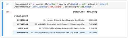
The approximation results are sorted by item descending rating which indicates the magnitude of the recommendation. In this case the top recommendation for the customer is:

• CH Hanson 0 Stud 4 Sure Magnetic Stud Finder

4. t-SNE Visualization

In this section we will discuss a notebook that uses the SVD results saved to the svd_cust_vec and svd_item_vec tables to generate a visualization that uses multiple algorithms to gain insights into the data. A summary of this diagram was discussed in the Concepts section.

The visualization is constructed by the workflow shown below that starts with a sparse rating matrix and ends with a 2D or 3D visualization. We take the SVD results from the previous sections and leverage k-means for clustering and t-SNE for additional dimensional reduction.

The SVD algorithm produces customer vectors and product vectors that are saved to tables. The k-means clustering algorithm takes the customer vectors and produces centroids for the clusters along with labels for the vectors that indicate what cluster they are a member of.

These results are saved to the svd_kmeans table. In this table we can see that each row has a cluster index, number of customers in the cluster, and centroid vector with components U0-U4.

Each centroid is the mean of a set of customer vectors and so we can it as if it was a customer vector and get an approximation of product ratings. We use SQL to compute dot products and get an approximation of each of the centroids.

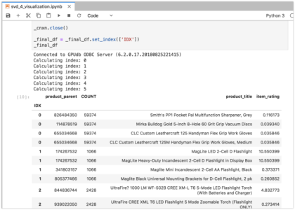
The resulting table (below) has a cluster index column in addition to product ratings and descriptions. By looking at the products we can manually determine a label for each of the clusters that will show in the legend of the visualization.

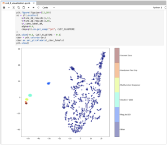
The next step is to plot the customer vectors We have a problem because they are 10 dimensional and our visualization is 2D. For this we leverage the t-SNE algorithm that can create a 2D representation of the 10D data. It does this by attempting to minimize the divergence between the points in the higher and lower dimensions.

We use a random sampling of 1000 points for this because the algorithm is computationally intensive. With the reduced number of points it can still take over 60 seconds to produce results. We combine the 2D points and k-means labels using the label to determine the color.

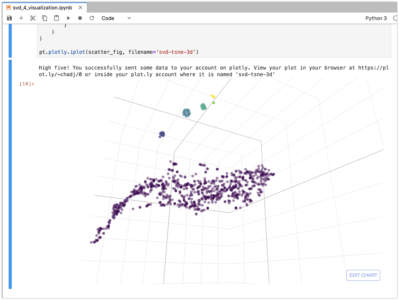
We can also use t-SNE to generate a 3D vectors using Plotly. The visualization below is a projection of the same data into 3 dimensions and similarities are apparent. For this to work you will need to sign up for a Plotly account and enter an API key in the code below.

# uncomment this and put your API key here#pt.tools.set_credentials_file(username='x', api_key='x')

Caveats

The examples given have some limitations that may need to be addressed before functioning in a real-world situation:

• The Amazon dataset we used told us nothing about similarities between products. For example grey and black flashlights that are otherwise identical are considered completely different products even though a customer may be equally interested in both of them. If we had additional product metadata we could combine these SKU’s and get more insights into purchasing preferences.
• If you used the Kinetica JupyterLab docker image for this tutorial then you are using the Intel build and not leveraging the GPU capabilities of PyTorch or Kinetica. Because of the computational and memory overhead the number of products were reduced to the top 500. For larger data sets powerful GPU accelerated hardware may be necessary.
• We did not represent the sparse matrix with a sparse datatype and so empty cells generate a lot of memory overhead.
• The PyTorch implementation of the SVD solver is not distributed and so solving the sparse matrix is limited to a single node. Distributed algorithms are available that can scale to much larger data sets.
• The examples given require that the entire matrix be re-solved when a change is made to the input data set. In some cases this is not acceptable an incremental approach is needed that can efficiently adapt to new data. There are incremental forms of SVD that can solve this problem.
• The solution that won the Netflix challenge was a modified version of SVD often called SVD++ that includes the concept of implicit feedback that considers the importance of which products a user rates as instead of only how the products were rated.

Conclusion

This tutorial has demonstrated a few significant applications of sparse data analysis on the Kinetica platform. Sparse data is common occurrence and many of the traditional methods of analysis can be biased by assumptions and lack of depth.

For example a non-ML product recommender could be biased by assumptions made by the designers. Customer purchasing groups could be identified by top-N “group by” queries but this would this fail to find previously unknown correlations between multiple purchases.

Hopefully these examples can inspire readers to get hands-on with more sophisticated ML analysis techniques and challenge themselves to find relevant use cases and bring new value to their business with the help of Kinetica as an ML platform.

Chad Juliano is a Principal Consultant at Kinetica.