In previous articles we have shown you how you can use Kinetica to collect geospatial streaming data from Meetup.com and visualize it using either Kinetica Reveal or a custom application connecting to the database using Javascript API.
These days, visualizing and basic statistical analysis is often not enough to give your company a competitive advantage. Artificial Intelligence and Machine learning (ML) techniques are often used to provide even deeper insights into your data and discover new patterns and knowledge.
Let’s do something interesting with our data as well. Something that could be very useful to event organizers is knowing how many people will actually show up at the event. Using ML and our RSVP records, we could train a model capable of predicting the number of people who confirm event attendance. Kinetica can help with this.
AI and ML algorithms often require a lot of computing power to train and your company needs to own a suitable infrastructure designed specifically for these purposes. Configuring and maintaining such infrastructure can be costly. Additionally you also have to move data between your database and AI/ML systems. This process can be time consuming.
What if, instead of building your machine learning cluster from scratch, you could utilize your database systems that are already up and running and contain all the data you want to use? This is exactly the approach offered by Kinetica.
Active Analytics Workbench
In version 7.0, a brand new Active Analytics Workbench (AAW) interface was added to the Kinetica platform.
Now with Kinetica, if your data scientist develops a model, you can easily import it into our Active Analytics Workbench with a few simple clicks. You can automatically deploy those models as containers in a batch, on demand, or in continuous mode—an easy way to incorporate machine learning into your application.
With the Kinetica Active Analytics Workbench, you can simply bring all of your analytics, register them as a container, and voila, all of the data orchestration and management is done for you. It’s the easiest way to build active analytical applications that incorporate machine learning.
As I mentioned, this tool allows you to easily deploy different machine learning models. Two options are available – you can either use Tensorflow or create a blackbox model as a Docker image with a specific interface.
As you already know Kinetica can utilize NVIDIA GPUs to greatly increase its performance. You can of course use this power for your ML models too. In our case though, we choose the CPU alternative, as we don’t have GPUs on our machine and the ML model itself is quite simple.
Predicting the number of yes responses
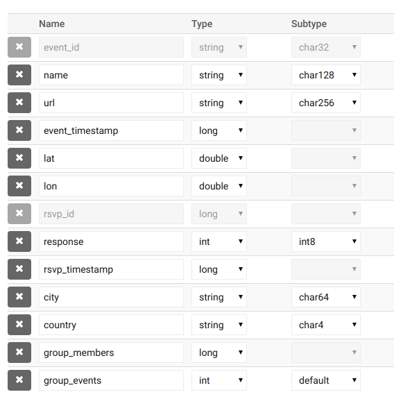
Before we get to use AAW, let’s talk a little about our prediction model. The model output is pretty obvious: we simply want the number of people which are going to say yes to our event. To make a prediction we also need to provide some input. Let’s review what data we have in our database:
Looking at the table structure, we could use the number of group members, number of previous group events, city and country to make a prediction. We also know the time of the event. From this we could extract the local day of week and the hour when the event starts. We have 6 input variables in total. Seems good so far.
Next, we need some data to train the model – we need to know how many people responded positively to previous events. To do this, we can simply group the responses in the table by event_id and get the sum of the response column values. If you recall, the response value is 1 for a positive response and a 0 for a negative response. By adding everything up, we simply get the number of yes responses.
Using this data we are going to train a simple neural network regressor. Since we are not using the GPU, the scikit-learn implementation will suffice. Additionally, Meetup RSVPs are generated in real time. We want to utilize this fact and update our model as we gather more and more data. This means that our prediction procedure will look like this:
-
- User provides input for prediction (country, city, day of week, hour, group events, group members);
-
- The prediction models updated the data we have collected since the last model update;
-
- Update model is used to make a prediction;
-
- Updated model is stored for later use;
- Predicted number of yes responses is returned to the user.
Storing the model in the database
To store and load our prediction models we are going to create a database table with the following structure:
table_structure = [
[‘model_id’, ‘int’, ‘primary_key’, ‘shard_key’],
[‘dump’, ‘bytes’],
[‘created_on’, ‘long’, ‘timestamp’],
[‘sample_cnt’, ‘long’],
[‘test_r2’, ‘double’],
[‘train_r2’, ‘double’]
]
The model itself is going to be stored in the dump column. For serialization and deserialization we use Python’s built-in pickle library. We also want to store some metadata: the number of new samples used to train and test R2 scores. These are used to evaluate our model. Put simply, the closer we are to 1.0, the better the model is.
Creating the AAW BlackBox model
As mentioned in the beginning, you can either use Tensorflow or Docker images to define an ML model in AAW. For our use case we chose the second option. This model type is called BlackBox.
To create a compatible Docker image, Kinetica provides a BlackBox Container SDK. In the simplest case, if you want to define a model using this SDK, all you have to do is to create a new Python module (file) and define a single function implementing the model. This function should accept one parameter: a dictionary containing input values and it should return a dictionary containing output values. In our case the input dictionary contains the following keys:
-
- city
-
- country
-
- day_of_week
-
- hour
-
- group_members
- group_events
On the other hand, the function returns a dictionary with just one key:
- predicted_yes_responses
Furthermore, we also modified the KineticaBlackBox class, so it provides some additional arguments to our model function – we need access to the database connection object since we are loading training data from the database and storing trained models. We also want to use the logger object created by the class in our model to report what’s happening.
If you want to know more about how the model works, feel free to check our repository.
After the model is implemented, we can modify the Dockerfile in the SDK code and add all required dependencies. Finally we change the Docker image URL in the release.sh file and run the script to build and publish the image. Our BlackBox image is available at https://hub.docker.com/r/profiq/kinetica-meetup-prediction.
Tip: You can host your Docker images for free on gitlab.com or hub.docker.com.
Adding a model in AAW
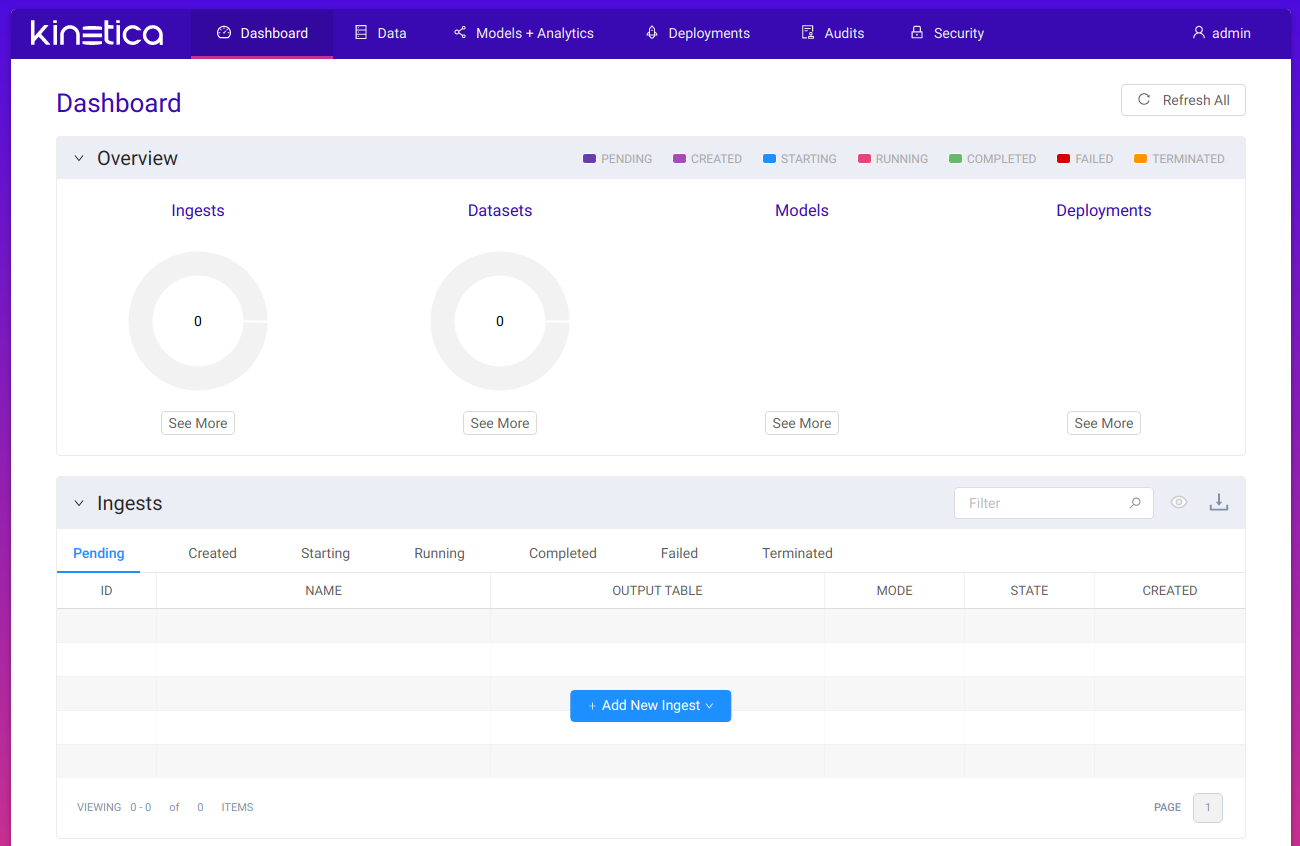
Our Docker image is ready and we can finally open the AAW interface to add our model to Kinetica. AAW is accessible through your browser on port 8070 of your Kinetica machine by default. After you log in with your admin username and password, we will get redirected to the AAW dashboard:
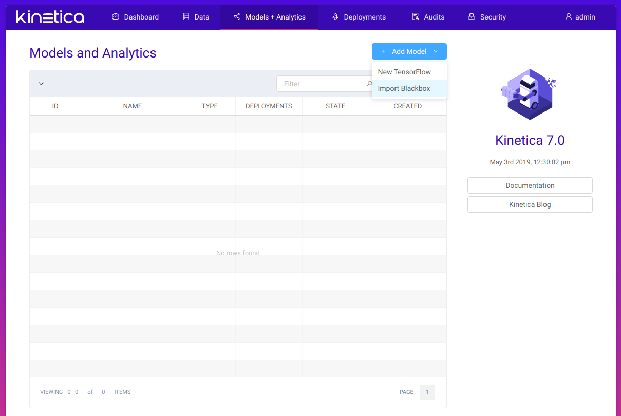
To add a model we click the Models + Analytics option from the top bar, then hover over the Add model button and finally select the Import Blackbox option:
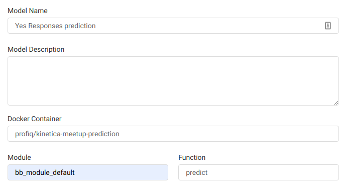
The input and output columns need to match the keys of the input and output dictionaries we already discussed:
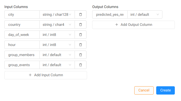
In our model, day of week is expected to be an integer – 0 for Monday, 6 for Sunday. Country is represented by its lowercase 2-letter ISO code.
After we define inputs and outputs, we can create the model. We are redirected to the model page:
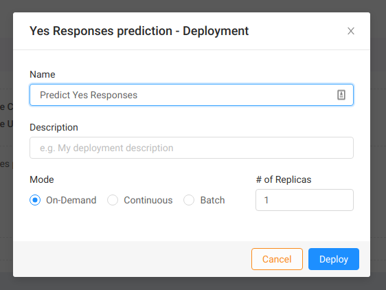
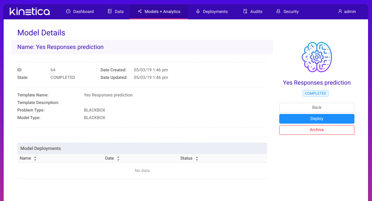 The model itself isn’t doing much right now. It needs to be deployed first. To do so, we click on the Deploy button on the right. In the dialog we enter the deployment’s name and select type of deployment. In this case we choose on-demand deployment. This allows us to ask the model for a single prediction whenever we want. We also want to deploy just one replica:
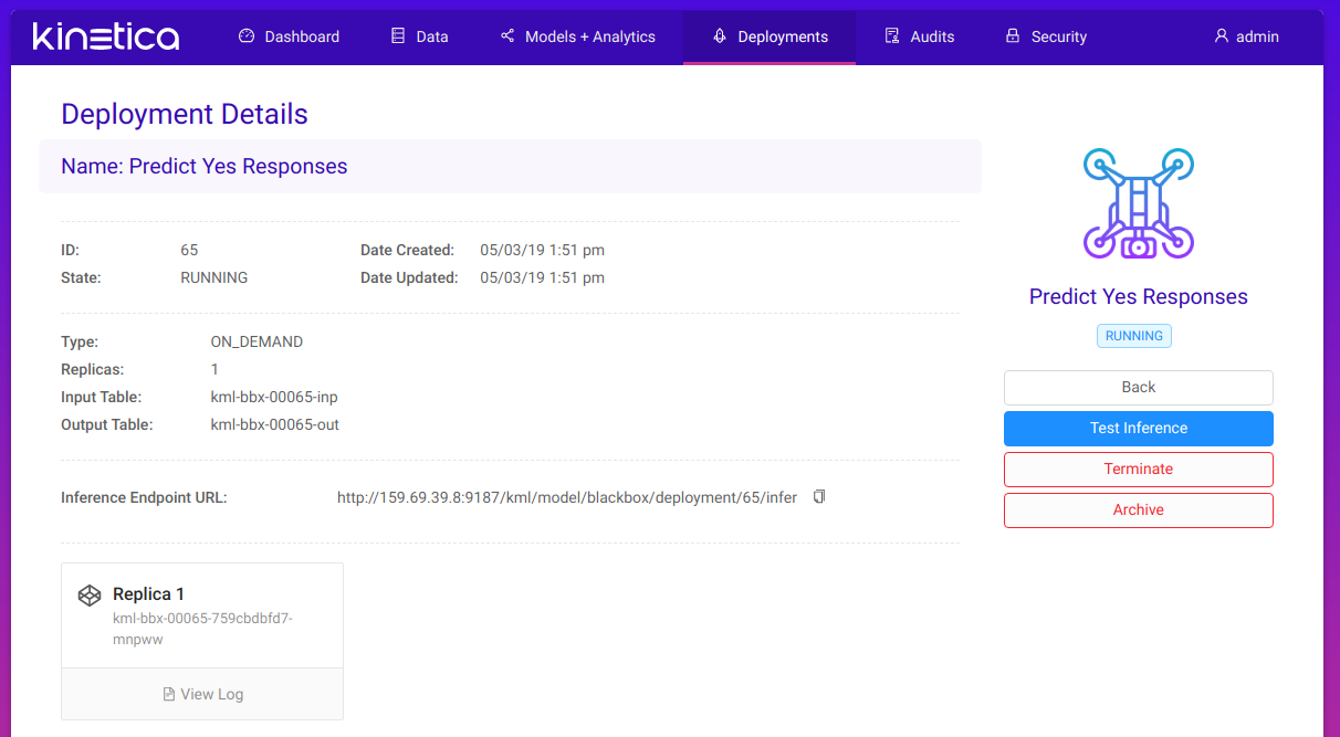
After we deploy the model we are redirected to the deployment page. Here we can see the status of the model instance, view logs from the actual Docker container, and terminate the deployment if it’s no longer needed.
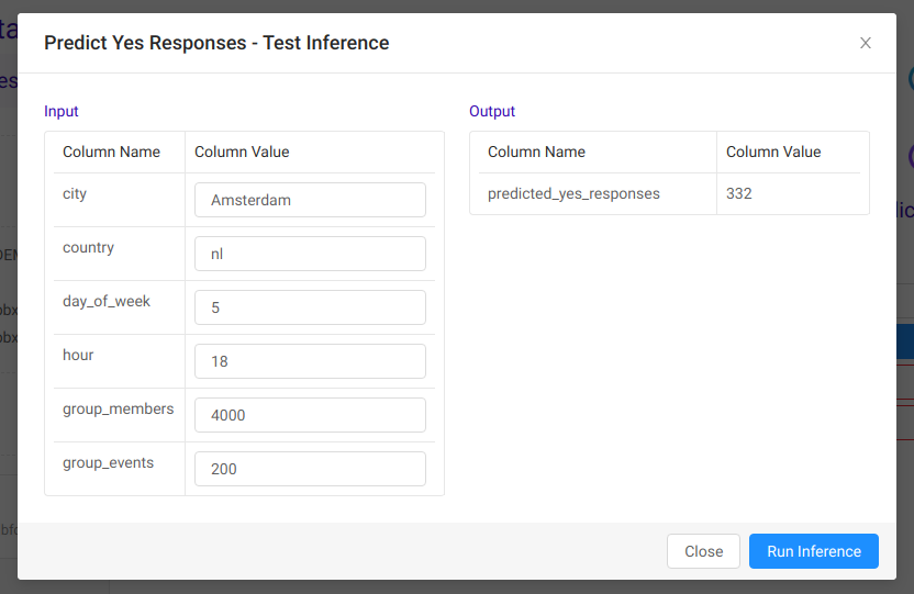
 Most importantly though, we can use the Test inference option to make a prediction. We simply enter the input values into the form and click the Run Inference button:
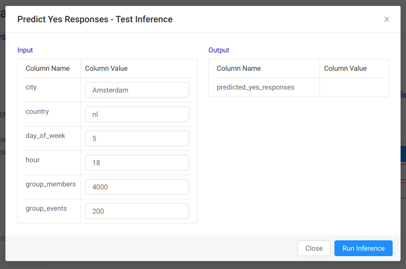 After a few seconds we have a result. We predicted that around 332 people can be expected to attend an event described by provided input values.

Conclusion
In this article we have shown you how Kinetica can help you with implementing advanced machine learning solutions. The brand new Active Analytics Workbench interface allows you to easily deploy Tensorflow models or custom Docker images allowing you to solve complex data science problems.
At Kinetica, as part of our active analytics platform, we’ve set out to solve the challenge of integrating your best algorithms and machine learning models seamlessly into your application in a way that will help you deliver real-time experiences, while at the same time giving you the corporate governance and ease of use that you need to scale. Try out our Active Analytics Workbench and see for yourself!
Throughout the series we highlighted some of the features of the Kinetica platform that make the lives of developers and data analysts easier when dealing with huge amounts of data. Fast data storage capable of utilizing NVIDIA GPUs for quick computations, Reveal the powerful visualization tool, the ability to deal with geospatial data, APIs for creating custom apps, and finally, machine learning and advanced data analysis tools. We hope after reading the series you will consider using Kinetica to tackle your next extreme data projects.
Disclaimer: We do not guarantee that the prediction model described in this guide will provide good results. Creation of a good regression model requires extended exploratory data analysis, preprocessing, and tweaking. In this case these steps are skipped and we focus on describing Active Analytics Workbench workflow and ML model implementation.
Check out the other blogs in this series:



 Using the form we provide a name for our model, URL of the Docker image as if we used it with the