Spatial operations from hours to minutes.

Q: How is Kinetica's geospatial engine different from PostGIS?

PostGIS is the gold standard for geospatial depth on a single-machine row-store. Kinetica matches PostGIS-style grammar with 150+ ST_ functions — and adds GPU-vectorized execution, parallel CPU dispatch, and a distributed shared-nothing architecture. The same SQL that hits a wall on PostGIS at 100M rows runs in seconds on Kinetica. The independent Radiant Advisors benchmark measured a 270× speedup on a 100M-trip geo-join workload.

Q: Does Kinetica run on GPU, CPU, or both?

Both — and the planner picks. Column-wide GIS work (point-in-polygon over a billion rows, server-side rendering, density surfaces) is routed to GPU lanes. Individual ST_ functions, graph solvers, and H3 grid operations run on parallel CPU. There's no manual hint required: same SQL, the substrate adapts to the shape of the workload.

Q: Is H3 indexing native, or do I need an extension?

Native. H3 functions ship as first-class SQL — H3_LATLNGTOCELL , H3_POLYGONTOCELLS , H3_GRIDDISK , H3_CELLTOPARENT , and the full Uber H3 family — with sixteen resolutions from continent to half-meter. No extension to install, no UDF library to package.

Q: Can I run spatiotemporal queries on moving objects?

Yes. A track is a first-class object — a sequence of points ordered by time, addressed by an ID column. ST_TRACKINTERSECTS matches tracks against geofences (with optional time tolerance), ST_TRACK_DWITHIN finds tracks within a space-time radius, and ST_LINESTRINGFROMORDEREDPOINTS materializes the line geometry. One table function replaces a streaming layer plus a spatial DB plus a graph engine.

Q: What rendering modes does the WMS endpoint support?

Six modes, all GPU-rendered server-side and returned as PNG over HTTP: raster (point clouds), cb_raster (class breaks), heatmap (60+ colormaps with log/sum/avg/count aggregation), contour (marching-squares isolines with IDW gridding), labels , and isochrones (graph-driven reachability surfaces). All six are also available as vector tiles via the /vts endpoint.

Q: How do spatial queries combine with graph queries?

In one SQL statement. Spatial geometries are valid graph weights — ST_LENGTH on a road segment is a travel-time weight when divided by speed. Build the graph with CREATE OR REPLACE GRAPH over a road network, then issue SHORTEST_PATH or render an isochrone via the WMS endpoint. The same engine that ran your point-in-polygon query just walked the graph and rendered the image.

GeospatialGPU + parallel CPUPostGIS grammarH3TracksServer-side render

150+ PostGIS-compatible functions, H3 indexing, track operators, and server-side map rendering — all in SQL, all on GPU.

Start FreeSQL · H3 · WKT · WMS · VTS

The Category

PostGIS is the richest geospatial library — but it's CPU-bound at scale. Kinetica runs the same SQL, 240x faster.

POSTGRES + POSTGIS

The richest function library — CPU-bound at scale.

Decades of development have made PostGIS the gold standard for geospatial depth. The cost: it's a row-store on CPUs. Point-in-polygon over hundreds of millions of rows hits a wall.

Deepest geospatial function library in OSS

Single-machine, single-core query execution

Performance falters on very large datasets

The Mechanism

Point-in-polygon over 100M rows skips the chunks it can — then vectorizes the rest. Pruned first, dispatched once, not 100 million row iterations.

Execution model · 100M-row point-in-polygon

Row-by-row CPUChunk-skip → vectorized GPU + CPU

CPU · row-by-row execution

One function call per row

i=0 · ST_CONTAINS(poly, point)

i=1 · ST_CONTAINS(poly, point)

i=2 · ST_CONTAINS(poly, point)

i=3 · ST_CONTAINS(poly, point)

i=4 · ST_CONTAINS(poly, point)

… 100,000,000 iterations

processing 9.8M / 100M

Wall clock

Grows linearly with row count.

Every row pays the full function cost.

Chunk-skip → vectorized · GPU + parallel CPU

Prune by chunk, then dispatch once across N lanes

① CHUNK SKIP · min/max range vs polygon bbox

Each chunk = 8M rows with cached min/max ranges. Chunks outside the polygon's bounding box are skipped before ST_CONTAINS runs — the predicate only touches candidate chunks.

② VECTORIZE · function dispatched once · ranks → TOMs → lanes

TOM₀

TOM₁

TOM₂

TOM₃

TOM₄

TOM₅

TOM₆

TOM₇

one rank per GPU · multiple TOMs per rank …

candidate rows · done

Wall clock

Skipped chunks cost nothing; survivors run in parallel.

Sublinear when the query is selective.

How it works

Columnar storage touches only the columns in the query; horizontal chunks (8M rows, default) carry per-column min/max metadata so chunks that can't contain a match are skipped. The survivors are dispatched once and vectorized across ranks and TOMs — GPU for rendering and most GIS functions, parallel CPU for the st_functions that run there.

Source: Kinetica Core Database 7.1 — vertical/horizontal grouping & GPU/CPU query orchestration.

Field report

“Spatial operations that typically take several hours on traditional databases can now be completed within a couple of minutes, allowing Foursquare to push the boundaries of what's possible with SQL in the geospatial domain.”

Foursquare on building the FSQ DB geospatial compute layer with Kinetica

The Numbers

Independent benchmark. Same hardware. 100M rows.

Geo Filter & Sum

100M trips · less is better

3.4×faster

How long were rides originating in this area? STXY_INTERSECTS + aggregation.

Kinetica16.0 s

PostGIS54.1 s

rowsKineticaPostGIS10M2.83 s7.29 s50M8.50 s26.78 s100M16.02 s54.13 s

Geo Join & Count

100M trips · less is better

270×faster

How many trips originated and ended in an area? STXY_INTERSECTS over both endpoints.

Kinetica64 s

PostGIS17,285 s (~4.8 hrs)

rowsKineticaPostGIS10M8.84 s3,779 s50M30.4 s11,113 s100M64 s17,285 s

Geo Join & Temporal Filter

100M trips · less is better

34×faster

Trips intersecting an area where duration < 10 min — joined geometry + time predicate.

Kinetica0.27 s

PostGIS9.28 s

rowsKineticaPostGIS10M0.14 s4.76 s50M0.23 s13.62 s100M0.27 s9.28 s

Methodology

Source: Radiant Advisors Independent Space & Time Database Benchmark, Q3 2022.

Workload: 100M Citi Bike trips. Hardware: both systems provisioned with 192 CPUs and 2 TB premium SSD —

Kinetica distributed across 4× ESDv2 nodes; PostGIS on a single Azure M192. Equivalent compute, distinct topology.

Full SQL and data on the Radiant Advisors GitHub →

The Toolkit

Geometry. Hex grids. Tracks. Maps. One toolbox.

Geometry · ST_*

150+ functions

Full PostGIS-style geometry library.

Predicates, measurements, constructions, set operations, transforms. Plus enhanced STXY_* variants for raw x/y columns.

SELECT id
FROM points
WHERE STXY_CONTAINS(
  zone_geom, lon, lat
) = 1;

ST_CONTAINS · ST_INTERSECTS · ST_DWITHIN · ST_BUFFER · ST_AREA · ST_LENGTH · ST_CENTROID · ST_DISTANCE · ST_UNION · ST_CONVEXHULL

H3 grids · H3_*

native indexing

Uber's hex tessellation, in SQL.

Convert points and polygons to H3 cells, walk parent and child levels, take grid disks and rings. Sixteen resolutions, continent to half-meter.

SELECT
  H3_LATLNGTOCELL(
    lat, lon, 9
  ) AS cell,
  COUNT(*)
FROM events
GROUP BY cell;

H3_LATLNGTOCELL · H3_POLYGONTOCELLS · H3_GRIDDISK · H3_GRIDRING · H3_CELLTOPARENT · H3_CELLTOCHILDREN · H3_CELLTOBOUNDARY

Tracks · ST_TRACK*

spatial × temporal

Time-aware moving objects.

A track is a sequence of points ordered by time — flights, vehicles, ships. Match tracks against geofences or find tracks within a space-time tolerance.

SELECT *
FROM TABLE(
  ST_TRACKINTERSECTS(
    TRACK_TABLE => ...,
    GEOFENCE_TABLE => ...
  )
);

ST_TRACK_DWITHIN · ST_TRACKINTERSECTS · ST_TRACKLENGTH · ST_TRACKDURATION · ST_LINESTRINGFROMORDEREDPOINTS

Visualization · /wms · /vts

GPU rendering

Render the map in the database.

Issue an HTTP request, get back a PNG. Six rendering modes covering point clouds, choropleths, density surfaces, and route reachability.

GET /wms?REQUEST=
  'GetMap'
  &STYLES='heatmap'
  &LAYERS=trips
  &BBOX=...

raster · cb_raster · heatmap (60+ colormaps) · contour (isolines) · labels · isochrones · vector tile service (VTS)

The Hybrid

Moving objects, geofences, and time windows in one SQL table function — no streaming layer, no graph DB, no glue code.

Tracks · Geofences · Time tolerance

downtown_fenceairport_fencematched track

SQL · flights_through_geofences.sqlST_TRACKINTERSECTS

-- Find every flight that crosses
-- a geofence within a time window.
-- One table function. One query.

SELECT *
FROM TABLE(
  ST_TRACKINTERSECTS(
    TRACK_TABLE       => INPUT_TABLE(flights),
    TRACK_ID_COLUMN    => 'flight_id',
    TRACK_X_COLUMN     => 'lon',
    TRACK_Y_COLUMN     => 'lat',
    TRACK_ORDER_COLUMN => 'flight_time',
    GEOFENCE_TABLE      => INPUT_TABLE(geofences),
    GEOFENCE_ID_COLUMN  => 'fence_name',
    GEOFENCE_WKT_COLUMN => 'fence_wkt'
  )
)
ORDER BY flight_id, fence_name;

↑ Spatial + temporal + label-aware. No streaming layer, no graph DB.

And because graph is native

Travel-time curves over a road network — produced by the same engine.

Isochrone · spatial × graph

5 min15 min30 min

One HTTP GET returns a PNG. Style with URL parameters; restyle without re-querying.

URL · isochrone_render.sh/wms · isochrones

# A graph weighted by ST_LENGTH
CREATE OR REPLACE GRAPH roads (
  EDGES => INPUT_TABLES(
    SELECT
      shape AS EDGE_WKTLINE,
      ST_LENGTH(shape, 1) / speed
        AS WEIGHTS_VALUESPECIFIED
    FROM road_network
  )
);

# One HTTP call returns a PNG
GET /wms?
  STYLES=isochrones
  &GRAPH_NAME=roads
  &SOURCE_NODE='POINT(-122 47)'
  &NUM_LEVELS=3
  &COLORMAP=viridis

Graph weighted by ST_LENGTH · one HTTP call returns the rendered image

The Visualization

Render the map in the database.

Server-rendered heatmap of 100M Citi Bike trips across Manhattan, with density blooming in plasma colors over Midtown and downtown.

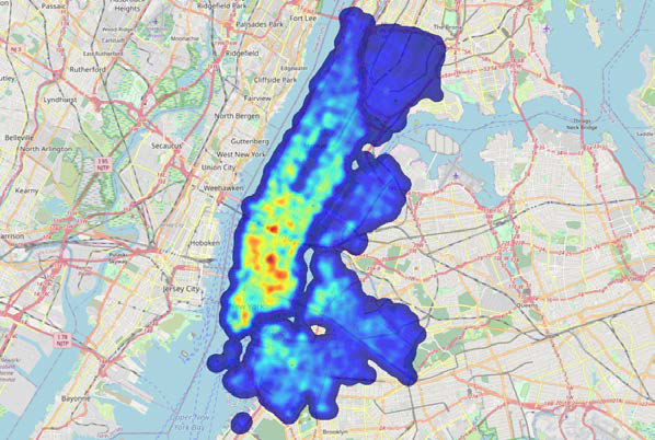
Density surfaces from millions of points.

Per-pixel aggregation directly over the source table. Sum, count, average, log-scaled — paired with any of 60+ colormaps from viridis to magma to inferno. Shown: 100M Citi Bike trips, rendered server-side in under one second, delivered as a PNG over HTTP.

VAL_ATTR = count / sum / avg / min / max / log(...)
COLORMAP: 60+ built in
BLUR_RADIUS · MIN_LEVEL · MAX_LEVEL parameterized

Engineering note

Pre-baking tiles is the wrong layer. The renderer should sit next to the data, not downstream of it — the map is finished when it leaves the database. One HTTP GET returns the rendered PNG; style with URL parameters and restyle without re-querying.

— Kinetica engineering · WMS rendering of 2.3B NYC taxi pickups · sub-second response from a single GET, vs. ~12 sec to ship raw points to a client renderer and rasterize there

Every dialect of geospatial.
One vectorized engine.

Start Free Read the docs

Frequently asked questions

How is Kinetica's geospatial engine different from PostGIS?

PostGIS is the gold standard for geospatial depth on a single-machine row-store. Kinetica matches PostGIS-style grammar with 150+ ST_ functions — and adds GPU-vectorized execution, parallel CPU dispatch, and a distributed shared-nothing architecture. The same SQL that hits a wall on PostGIS at 100M rows runs in seconds on Kinetica. The independent Radiant Advisors benchmark measured a 270× speedup on a 100M-trip geo-join workload.

Does Kinetica run on GPU, CPU, or both?

Both — and the planner picks. Column-wide GIS work (point-in-polygon over a billion rows, server-side rendering, density surfaces) is routed to GPU lanes. Individual ST_ functions, graph solvers, and H3 grid operations run on parallel CPU. There's no manual hint required: same SQL, the substrate adapts to the shape of the workload.

Is H3 indexing native, or do I need an extension?

Native. H3 functions ship as first-class SQL — H3_LATLNGTOCELL, H3_POLYGONTOCELLS, H3_GRIDDISK, H3_CELLTOPARENT, and the full Uber H3 family — with sixteen resolutions from continent to half-meter. No extension to install, no UDF library to package.

Can I run spatiotemporal queries on moving objects?

Yes. A track is a first-class object — a sequence of points ordered by time, addressed by an ID column. ST_TRACKINTERSECTS matches tracks against geofences (with optional time tolerance), ST_TRACK_DWITHIN finds tracks within a space-time radius, and ST_LINESTRINGFROMORDEREDPOINTS materializes the line geometry. One table function replaces a streaming layer plus a spatial DB plus a graph engine.

What rendering modes does the WMS endpoint support?

Six modes, all GPU-rendered server-side and returned as PNG over HTTP: raster (point clouds), cb_raster (class breaks), heatmap (60+ colormaps with log/sum/avg/count aggregation), contour (marching-squares isolines with IDW gridding), labels, and isochrones (graph-driven reachability surfaces). All six are also available as vector tiles via the /vts endpoint.

How do spatial queries combine with graph queries?

In one SQL statement. Spatial geometries are valid graph weights — ST_LENGTH on a road segment is a travel-time weight when divided by speed. Build the graph with CREATE OR REPLACE GRAPH over a road network, then issue SHORTEST_PATH or render an isochrone via the WMS endpoint. The same engine that ran your point-in-polygon query just walked the graph and rendered the image.

Spatial operations from hours to minutes.

The richest function library — CPU-bound at scale.

Geo Filter & Sum

Geo Join & Count

Geo Join & Temporal Filter

Full PostGIS-style geometry library.

Uber's hex tessellation, in SQL.

Time-aware moving objects.

Render the map in the database.

Travel-time curves over a road network — produced by the same engine.

Density surfaces from millions of points.

Every dialect of geospatial.One vectorized engine.

Frequently asked questions

Every dialect of geospatial.
One vectorized engine.